One of the exciting aspects of aggregations are how easily they are converted into charts and graphs. In this chapter, we are focusing on various analytics that we can wring out of our example dataset. We will also demonstrate the types of charts aggregations can power.

The histogram bucket is particularly useful. Histograms are essentially bar charts, and if you’ve ever built a report or analytics dashboard, you undoubtedly had a few bar charts in it. The histogram works by specifying an interval. If we were histogramming sale prices, you might specify an interval of 20,000. This would create a new bucket every $20,000. Documents are then sorted into buckets.

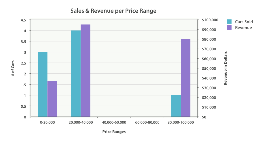
For our dashboard, we want to know how many cars sold in each price range. We would also like to know the total revenue generated by that price bracket. This is calculated by summing the price of each car sold in that interval.

To do this, we use a histogram and a nested sum metric:

GET /cars/transactions/_search
{
   "size" : 0,
   "aggs":{
      "price":{
         "histogram":{ 
            "field": "price",
            "interval": 20000
         },
         "aggs":{
            "revenue": {
               "sum": { 
                 "field" : "price"
               }
             }
         }
      }
   }
}

As you can see, our query is built around the price aggregation, which contains a histogram bucket. This bucket requires a numeric field to calculate buckets on, and an interval size. The interval defines how "wide" each bucket is. An interval of 20000 means we will have the ranges [0-19999, 20000-39999, ...].

Next, we define a nested metric inside the histogram. This is a sum metric, which will sum up the price field from each document landing in that price range. This gives us the revenue for each price range, so we can see if our business makes more money from commodity or luxury cars.

And here is the response:

{
...
   "aggregations": {
      "price": {
         "buckets": [
            {
               "key": 0,
               "doc_count": 3,
               "revenue": {
                  "value": 37000
               }
            },
            {
               "key": 20000,
               "doc_count": 4,
               "revenue": {
                  "value": 95000
               }
            },
            {
               "key": 80000,
               "doc_count": 1,
               "revenue": {
                  "value": 80000
               }
            }
         ]
      }
   }
}

The response is fairly self-explanatory, but it should be noted that the histogram keys correspond to the lower boundary of the interval. The key 0 means 0-19,999, the key 20000 means 20,000-39,999, and so forth.

Graphically, you could represent the preceding data in the histogram shown in Figure 35, “Sales and Revenue per price bracket”.

Figure 35. Sales and Revenue per price bracket

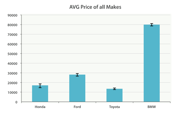
Of course, you can build bar charts with any aggregation that emits categories and statistics, not just the histogram bucket. Let’s build a bar chart of the top 10 most popular makes, and their average price, and then calculate the standard error to add error bars on our chart. This will use the terms bucket and an extended_stats metric:

GET /cars/transactions/_search
{
  "size" : 0,
  "aggs": {
    "makes": {
      "terms": {
        "field": "make",
        "size": 10
      },
      "aggs": {
        "stats": {
          "extended_stats": {
            "field": "price"
          }
        }
      }
    }
  }
}

This will return a list of makes (sorted by popularity) and a variety of statistics about each. In particular, we are interested in stats.avg, stats.count, and stats.std_deviation. Using this information, we can calculate the standard error:

std_err = std_deviation / count

This will allow us to build a chart like Figure 36, “Average price of all makes, with error bars”.

Figure 36. Average price of all makes, with error bars